
AWS re:Invent 2019 上,SageMaker 发布不少新功能,其中包括:Deep Graph Library 支持,机器学习训练流程管理能力(Experiment),自动机器学习工具 Autopilot,数据处理和模型评估的管理(Processing),模型自动监控工具 Monitor,模型训练过程的调试工具 Debugger,ML 场景下的 IDE Studio。这篇文章介绍并分析了这些新特性的功能,同时夹杂一点个人对这些特性的看法和观点。
Deep Graph Library 支持
Deep Graph Library(以下称作 DGL) 是一个用来构建 GNN 的 Python 库。DGL 目前支持 PyTorch 和 MXNet,它为 GNN 的构建提供了高层的 API。
import dgl
import torch as th

g = dgl.DGLGraph()
g.add_nodes(5)                          # add 5 nodes
g.add_edges([0, 0, 0, 0], [1, 2, 3, 4]) # add 4 edges 0->1, 0->2, 0->3, 0->4
g.ndata['h'] = th.randn(5, 3)           # assign one 3D vector to each node
g.edata['h'] = th.randn(4, 4)           # assign one 4D vector to each edge
上面的示例来自 DGL,其构建了一个简单的 GNN 网络,它对 GCN 等都有对应的支持。目前 SageMaker 通过其 Estimator 接口支持发起一次 DGL 训练。这一特性并无太多值得称道之处,算是一个常规的特性。
机器学习训练管理能力(Experiment)
众所周知,机器学习的模型训练是一个迭代的过程。对于一个模型的训练,往往有多次的调参-训练的迭代。Experiment 就是对这一迭代过程的抽象。在介绍训练之前,首先介绍一下 Trial。Trial 是一次训练的过程。其中包括数据预处理,模型训练,模型评估等。而 Experiment,是由多个 Trial 组成的一个集合,比如一组相关的训练任务等。因此 Experiment 跟 Google Vizier 中的 Study,Katib 中的 Experiment 概念类似。
利用 SageMaker 提供的 SDK,Experiment 可以发起多次 Trial,并且提供一些数据的比对等功能。
from smexperiments.experiment import Experiment

# Create experiment.
mnist_experiment = Experiment.create(
    experiment_name="mnist-hand-written-digits-classification",
    description="Classification of mnist hand-written digits",
    sagemaker_boto_client=sm)

# Create trials
for i, num_hidden_channel in enumerate([2, 5, 10, 20, 32]):
    trial_name = f"cnn-training-job-{num_hidden_channel}-hidden-channels-{int(time.time())}"
    cnn_trial = Trial.create(
        trial_name=trial_name,
        experiment_name=mnist_experiment.experiment_name,
        sagemaker_boto_client=sm,
    )
    cnn_trial.add_trial_component(tracker.trial_component)

    cnn_training_job_name = "cnn-training-job-{}".format(int(time.time()))

    # Create one PyTorch or Tensorflow job.
    estimator = PyTorch(
        entry_point='mnist.py',
        role=role,
        sagemaker_session=sess,
        framework_version='1.1.0',
        train_instance_count=1,
        train_instance_type='ml.p3.2xlarge',
        hyperparameters={
            'hidden_channels': num_hidden_channels
        },
        metric_definitions=[
            {'Name':'train:loss', 'Regex':'Train Loss: (.*?);'},
            {'Name':'test:loss', 'Regex':'Test Average loss: (.*?),'},
            {'Name':'test:accuracy', 'Regex':'Test Accuracy: (.*?)%;'}
        ]
    )

    # Training.
    estimator.fit(
        inputs={'training': inputs},
        job_name=cnn_training_job_name,
        experiment_config={
            "ExperimentName": mnist_experiment.experiment_name,
            "TrialName": cnn_trial.trial_name,
            "TrialComponentDisplayName": "Training",
        }
    )
上述代码是一次完整的训练过程。这次训练暴力搜索了 num_hidden_channel 的取值,并且所有的训练都归属于一个 Experiment。可以看到,其中的概念与 katib Experiment 非常类似。不过其采取的思路与 NNI 更相似,为用户提供了一个 SDK。这样的方式对用户的代码有一定的侵入性。
自动机器学习工具 Autopilot
SageMaker 之前已经有了一个做模型调优的功能 Model Tuning,它支持进行超参数优化。而新退出的这一功能 Autopilot,支持更多的特性:
- 支持 tabular 格式的输入,可以自动地进行模型输入的预处理工作
- 传统机器学习算法的自动模型选择(Automatic algorithm selection)
- 自动超参数优化
- 分布式训练
- 自动的集群大小调整
通过下面的代码,就可以发起一次基于 Autopilot 的训练。看上去就跟 autosklearn 非常接近。
auto_ml_job_name = 'automl-dm-' + timestamp_suffix
print('AutoMLJobName: ' + auto_ml_job_name)

sm.create_auto_ml_job(AutoMLJobName=auto_ml_job_name,
                      InputDataConfig=input_data_config,
                      OutputDataConfig=output_data_config,
                      RoleArn=role)

candidates = sm.list_candidates_for_auto_ml_job(AutoMLJobName=auto_ml_job_name, SortBy='FinalObjectiveMetricValue')['Candidates']

model_arn = sm.create_model(Containers=best_candidate['InferenceContainers'],
                            ModelName=model_name,
                            ExecutionRoleArn=role)

ep_config = sm.create_endpoint_config(EndpointConfigName = epc_name,
                                      ProductionVariants=[{'InstanceType':'ml.m5.2xlarge',
                                                           'InitialInstanceCount':1,
                                                           'ModelName':model_name,
                                                           'VariantName':variant_name}])

create_endpoint_response = sm.create_endpoint(EndpointName=ep_name,
                                              EndpointConfigName=epc_name)
训练一共会被分为如下步骤:
- 数据切分,划分为训练集和验证集
- 数据分析,推荐合理的流水线(应该是算法的意思)
- 特征工程,其中包括数据转换等
- 选择合适的流水线,调整超参数
除此之外,Autopilot 会生成两个 Jupyter Notebook:
job = sm.describe_auto_ml_job(AutoMLJobName=auto_ml_job_name)
job_data_notebook = job['AutoMLJobArtifacts']['DataExplorationNotebookLocation']
job_candidate_notebook = job['AutoMLJobArtifacts']['CandidateDefinitionNotebookLocation']

print(job_data_notebook)
print(job_candidate_notebook)

s3://<PREFIX_REMOVED>/notebooks/SageMakerAutopilotCandidateDefinitionNotebook.ipynb
s3://<PREFIX_REMOVED>/notebooks/SageMakerAutopilotDataExplorationNotebook.ipynb
这两个 notebook 中的第一个记录了搜索到的候选模型的一些信息,而且所有的代码都是可用的。第二个记录了数据集相关的信息,不确定有没有特征工程有关的内容。
总体来说,是一个主打自动模型选择的功能,这一功能在传统机器学习算法领域会更有价值。
数据处理和模型评估的管理
在模型训练的流水线中,数据的准备工作是比较麻烦的。SageMaker 基于 sklearn 的 data transform 功能,提供了一种内置的数据处理功能的支持。
from sagemaker.sklearn.processing import SKLearnProcessor
sklearn_processor = SKLearnProcessor(framework_version='0.20.0',
                                     role=role,
                                     instance_count=1,
                                     instance_type='ml.m5.xlarge')

from sagemaker.processing import ProcessingInput, ProcessingOutput
sklearn_processor.run(
    code='preprocessing.py',
    # arguments = ['arg1', 'arg2'],
    inputs=[ProcessingInput(
        source='dataset.csv',
        destination='/opt/ml/processing/input')],
    outputs=[ProcessingOutput(source='/opt/ml/processing/output/train'),
        ProcessingOutput(source='/opt/ml/processing/output/validation'),
        ProcessingOutput(source='/opt/ml/processing/output/test')]
)
上述代码是其中的输入输出配置。本质上,它是利用容器来实现的,在 SDK 定义的函数中,用户需要指定运行的代码文件,输入和输出,就可以进行标准化的处理。其中 preprocessing.py 就是用户提供的预处理代码:
import pandas as pd
from sklearn.model_selection import train_test_split
# Read data locally
df = pd.read_csv('/opt/ml/processing/input/dataset.csv')
# Preprocess the data set
downsampled = apply_mad_data_science_skills(df)
# Split data set into training, validation, and test
train, test = train_test_split(downsampled, test_size=0.2)
train, validation = train_test_split(train, test_size=0.2)
# Create local output directories
try:
    os.makedirs('/opt/ml/processing/output/train')
    os.makedirs('/opt/ml/processing/output/validation')
    os.makedirs('/opt/ml/processing/output/test')
except:
    pass
# Save data locally
train.to_csv("/opt/ml/processing/output/train/train.csv")
validation.to_csv("/opt/ml/processing/output/validation/validation.csv")
test.to_csv("/opt/ml/processing/output/test/test.csv")
print('Finished running processing job')
基本来说,是一个对容器的应用。值得一提的是,Amazon 对于资源采取了简化的处理,分成了大中小等不同资源容量的机器,这里用的就是 ml.m5.xlarge。这种思路值得参考,它可以简化用户申请资源的配置选择,但是也一定程度上限制了用户的自由。
既然是使用容器来实现的,这一功能同样支持自定义容器,其中差异就是需要提供一个镜像的路径。
from sagemaker.processing import ScriptProcessor
script_processor = ScriptProcessor(image_uri='123456789012.dkr.ecr.us-west-2.amazonaws.com/sagemaker-spacy-container:latest',
                role=role,
                instance_count=1,
                instance_type='ml.m5.xlarge')
模型服务自动监控工具
模型服务上线后,如何对它的效果和请求进行分析,是一个困难的问题。模型服务自动监控功能,就是通过对上线的服务进行监控和分析,来更好的了解模型服务情况。它的功能可以概括为:
- 查看模型服务的历史输入输出
- 查看模型服务的表现和统计数据
其中对数据的最简单的观察就是查看输入和输出,DataCaptureConfig 的配置支持这一特性:
data_capture_configuration = {
    "EnableCapture": True,
    "InitialSamplingPercentage": 100,
    "DestinationS3Uri": s3_capture_upload_path,
    "CaptureOptions": [
        { "CaptureMode": "Output" },
        { "CaptureMode": "Input" }
    ],
    "CaptureContentTypeHeader": {
       "CsvContentTypes": ["text/csv"],
       "JsonContentTypes": ["application/json"]
}
create_endpoint_config_response = sm_client.create_endpoint_config(
    EndpointConfigName = endpoint_config_name,
    ProductionVariants=[{
        'InstanceType':'ml.m5.xlarge',
        'InitialInstanceCount':1,
        'InitialVariantWeight':1,
        'ModelName':model_name,
        'VariantName':'AllTrafficVariant'
    }],
    DataCaptureConfig = data_capture_configuration)
在利用 DataCaptureConfig 创建好 Endpoint 后,可以查看其历史输入输出:
    "endpointInput":{
        "observedContentType":"text/csv",
        "mode":"INPUT",
        "data":"132,25,113.2,96,269.9,107,229.1,87,7.1,7,2,0,0,0,0,0,0,0,0,0,0,0,0,0,0,0,0,0,0,0,1,0,0,0,0,0,0,0,0,0,0,0,0,0,0,0,0,0,0,0,0,0,0,0,0,0,0,0,0,0,0,0,0,1,0,1,0,0,1",
        "encoding":"CSV"
     },
     "endpointOutput":{
        "observedContentType":"text/csv; charset=utf-8",
        "mode":"OUTPUT",
        "data":"0.01076381653547287",
        "encoding":"CSV"}
     },
    "eventMetadata":{
        "eventId":"6ece5c74-7497-43f1-a263-4833557ffd63",
        "inferenceTime":"2019-11-22T08:24:40Z"},
        "eventVersion":"0"}
除了简单的输入和输出之外,可以通过 S3 上的三个对象 constraints.json,statistics.json 和 constraints_violations.json 查看更抽象的数据分析结果:
{
  "version" : 0.0,
  "features" : [ {
    "name" : "Churn",
    "inferred_type" : "Integral",
    "completeness" : 1.0
  }, {
    "name" : "Account Length",
    "inferred_type" : "Integral",
    "completeness" : 1.0
  }
  ]
}
比如 constraints.json 会显示推导的数据的类型等信息。而下列的 statistics.json 展示了数据的分布情况和统计信息。
{
    "name" : "Day Mins",
    "inferred_type" : "Fractional",
    "numerical_statistics" : {
      "common" : {
        "num_present" : 2333,
        "num_missing" : 0
      },
      "mean" : 180.22648949849963,
      "sum" : 420468.3999999996,
      "std_dev" : 53.987178959901556,
      "min" : 0.0,
      "max" : 350.8,
      "distribution" : {
        "kll" : {
          "buckets" : [ {
            "lower_bound" : 0.0,
            "upper_bound" : 35.08,
            "count" : 14.0
          }, {
            "lower_bound" : 35.08,
            "upper_bound" : 70.16,
            "count" : 48.0
          } ],
          "sketch" : {
            "parameters" : {
              "c" : 0.64,
              "k" : 2048.0
            },
            "data" : [ [ 178.1, 160.3 ...] ]
          }
        }
      }
    }
}
模型训练过程的调试工具
刚刚提到的模型服务的监控工具,而模型训练的过程调试也一直是个很困难的事情,传统软件开发有 gdb 等 debug 工具,而模型训练目前还没有完善的解决方案。SageMaker 提出了自己的尝试。Debugger 是一个 Python SDK。它提供了如下功能:
- 提供 TensorFlow 的 Session Hook,用来收集数据和训练指标,如权重,梯度等
- 提供 SaveConfig 配置,可以让用户指定收集频率
- (可选)Optimizer 的封装,用来支持收集梯度
- (可选)ReductionConfig,用来收集部分 Tensor 而不是全部
基本来说,就是围绕 SessionHook 的增强与优化,其示例如下。
reduc = smd.ReductionConfig(reductions=['mean'], abs_reductions=['max'], norms=['l1'])

hook = smd.SessionHook(out_dir=args.debug_path,
                       include_collections=['weights', 'gradients', 'losses'],
                       save_config=smd.SaveConfig(save_interval=args.debug_frequency),
                       reduction_config=reduc)

with tf.name_scope('initialize'):
    # 2-dimensional input sample
    x = tf.placeholder(shape=(None, 2), dtype=tf.float32)
    # Initial weights: [10, 10]
    w = tf.Variable(initial_value=[[10.], [10.]], name='weight1')
    # True weights, i.e. the ones we're trying to learn
    w0 = [[1], [1.]]
with tf.name_scope('multiply'):
    # Compute true label
    y = tf.matmul(x, w0)
    # Compute "predicted" label
    y_hat = tf.matmul(x, w)
with tf.name_scope('loss'):
    # Compute loss
    loss = tf.reduce_mean((y_hat - y) ** 2, name="loss")
    hook.add_to_collection('losses', loss)

optimizer = tf.train.AdamOptimizer(args.lr)
optimizer = hook.wrap_optimizer(optimizer)
optimizer_op = optimizer.minimize(loss)

hook.set_mode(smd.modes.TRAIN)

with tf.train.MonitoredSession(hooks=[hook]) as sess:
    for i in range(args.steps):
        x_ = np.random.random((10, 2)) * args.scale
        _loss, opt = sess.run([loss, optimizer_op], {x: x_})
        print (f'Step={i}, Loss={_loss}')
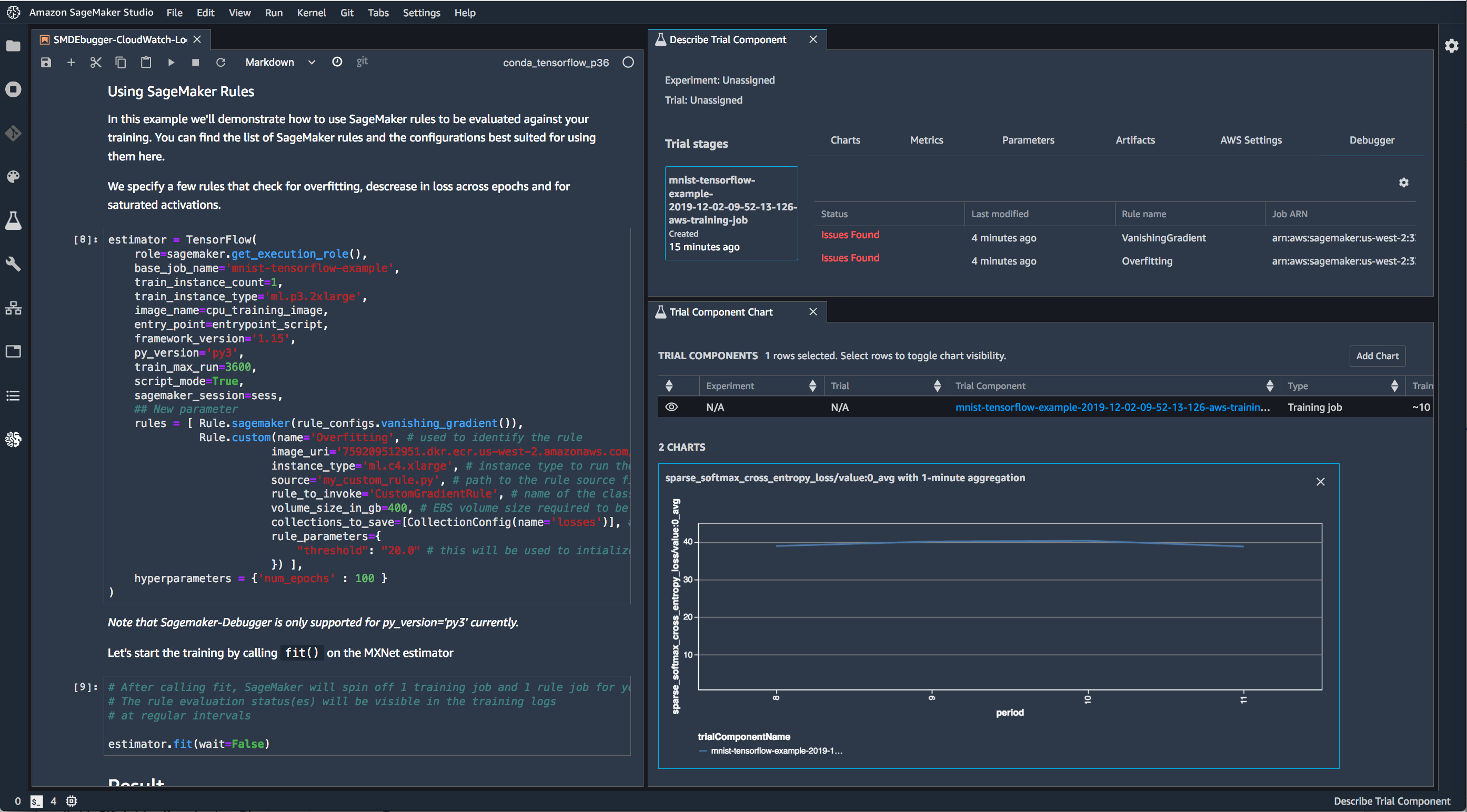
不过值得一提的是,在 SageMaker Debugger 的开源代码中,它给出了和博文不同的 API 使用方式:
import sagemaker as sm
from sagemaker.debugger import rule_configs, Rule, CollectionConfig

# Choose a built-in rule to monitor your training job
rule = Rule.sagemaker(
    rule_configs.exploding_tensor(),
    # configure your rule if applicable
    rule_parameters={"tensor_regex": ".*"},
    # specify collections to save for processing your rule
    collections_to_save=[
        CollectionConfig(name="weights"),
        CollectionConfig(name="losses"),
    ],
)

# Pass the rule to the estimator
sagemaker_simple_estimator = sm.tensorflow.TensorFlow(
    entry_point="script.py",
    role=sm.get_execution_role(),
    framework_version="1.15",
    py_version="py3",
    # argument for smdebug below
    rules=[rule],
)

sagemaker_simple_estimator.fit()
tensors_path = sagemaker_simple_estimator.latest_job_debugger_artifacts_path()

import smdebug as smd
trial = smd.trials.create_trial(out_dir=tensors_path)
print(f"Saved these tensors: {trial.tensor_names()}")
print(f"Loss values during evaluation were {trial.tensor('CrossEntropyLoss:0').values(mode=smd.modes.EVAL)}")
核心思路差不多,但是 API 变动挺大的,不知道是哪个版本更老一些。整体而言,是一个蛮有趣的功能,这种方式,通过对用户代码的侵入性修改,可以把训练过程的一些训练指标推送到远端。与其他如 MLFlow 等收集方式的实现相比,它直接提供了 SessionHook,稍微友好一些。
ML 场景下的 IDE
刚刚我们提到的 Experiment 特性,使得 SageMaker 有了自己独立的逻辑概念。而算法科学家喜爱的 Jupyter Notebook, 是不能原生地展示这些概念的,它并不能“理解”一个 Experiment 会与多个 Trials 相互关联。尽管 SageMaker 在文章里把 Motivation,但从我个人的角度,我认为最大的动机就是支持 Experiment 和 Trials 等新的特性。
所以,带着这样的思想,来看下它的 UI:
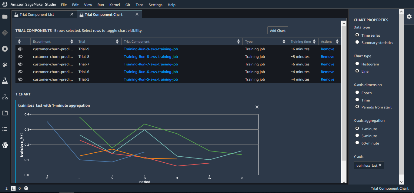
可以看到,基本都是围绕 Trial 和 Experiment 展开的。SageMaker 把 Jupyter 作为了本地模型开发的事实标准,对它进行了增强和修改,代表了业界的一种探索方向。不过我们也可以看到,有越来越多除了 Jupyter 之外的其他选择,所以这样的思路是否奏效,需要时间的检验了。
参考文档
License
- This article is licensed under CC BY-NC-SA 3.0.
- Please contact me for commercial use.